Tutorial 03 - Analysing Data Sets

In this tutorial we will be analysing the results of the calculations which we performed in the second tutorial. The tutorial will cover:

• comparing the estimated data set with the experimental data set.

• plotting the two data sets.

Note: If you are running this tutorial in google colab you will need to run a setup script instead of following the installation instructions:

# !wget https://raw.githubusercontent.com/openforcefield/openff-evaluator/master/docs/tutorials/colab_setup.ipynb
# %run colab_setup.ipynb

For the sake of clarity all warnings will be disabled in this tutorial:

import warnings
warnings.filterwarnings('ignore')
import logging
logging.getLogger("openforcefield").setLevel(logging.ERROR)

Loading the Data Sets

We will begin by loading both the experimental data set and the estimated data set:

from openff.evaluator.datasets import PhysicalPropertyDataSet

experimental_data_set_path = "filtered_data_set.json"
estimated_data_set_path = "estimated_data_set.json"

# If you have not yet completed the previous tutorials or do not have the data set files
# available, copies are provided by the framework:

# from openff.evaluator.utils import get_data_filename
# experimental_data_set_path = get_data_filename(
#     "tutorials/tutorial01/filtered_data_set.json"
# )
# estimated_data_set_path = get_data_filename(
#     "tutorials/tutorial02/estimated_data_set.json"
# )

experimental_data_set = PhysicalPropertyDataSet.from_json(experimental_data_set_path)
estimated_data_set = PhysicalPropertyDataSet.from_json(estimated_data_set_path)

if everything went well from the previous tutorials, these data sets will contain the density and \(H_{vap}\) of ethanol and isopropanol:

experimental_data_set.to_pandas().head()

	Temperature (K)	Pressure (kPa)	Phase	N Components	Component 1	Role 1	Mole Fraction 1	Exact Amount 1	Density Value (g / ml)	Density Uncertainty (g / ml)	EnthalpyOfVaporization Value (kJ / mol)	EnthalpyOfVaporization Uncertainty (kJ / mol)	Source
0	298.15	101.325	Liquid	1	CC(C)O	Solvent	1.0	None	0.78270	NaN	NaN	NaN	10.1016/j.fluid.2013.10.034
1	298.15	101.325	Liquid	1	CCO	Solvent	1.0	None	0.78507	NaN	NaN	NaN	10.1021/je1013476
2	298.15	101.325	Liquid + Gas	1	CCO	Solvent	1.0	None	NaN	NaN	42.26	0.02	10.1016/S0021-9614(71)80108-8
3	298.15	101.325	Liquid + Gas	1	CC(C)O	Solvent	1.0	None	NaN	NaN	45.34	0.02	10.1016/S0021-9614(71)80108-8

estimated_data_set.to_pandas().head()

	Temperature (K)	Pressure (kPa)	Phase	N Components	Component 1	Role 1	Mole Fraction 1	Exact Amount 1	Density Value (g / ml)	Density Uncertainty (g / ml)	EnthalpyOfVaporization Value (kJ / mol)	EnthalpyOfVaporization Uncertainty (kJ / mol)	Source
0	298.15	101.325	Liquid	1	CCO	Solvent	1.0	None	0.791767	0.000705	NaN	NaN	SimulationLayer
1	298.15	101.325	Liquid + Gas	1	CCO	Solvent	1.0	None	NaN	NaN	39.434820	0.170356	SimulationLayer
2	298.15	101.325	Liquid	1	CC(C)O	Solvent	1.0	None	0.804158	0.000680	NaN	NaN	SimulationLayer
3	298.15	101.325	Liquid + Gas	1	CC(C)O	Solvent	1.0	None	NaN	NaN	45.649979	0.234394	SimulationLayer

Extracting the Results

We will now compare how the value of each property estimated by simulation deviates from the experimental measurement.

To do this we will extract a list which contains pairs of experimental and evaluated properties. We can easily match properties based on the unique ids which were automatically assigned to them on their creation:

properties_by_type = {
    "Density": [],
    "EnthalpyOfVaporization": []
}

for experimental_property in experimental_data_set:

    # Find the estimated property which has the same id as the
    # experimental property.
    estimated_property = next(
        x for x in estimated_data_set if x.id == experimental_property.id
    )

    # Add this pair of properties to the list of pairs
    property_type = experimental_property.__class__.__name__
    properties_by_type[property_type].append((experimental_property, estimated_property))

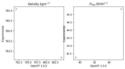
Plotting the Results

We will now compare the experimental results to the estimated ones by plotting them using matplotlib:

from matplotlib import pyplot

# Create the figure we will plot to.
figure, axes = pyplot.subplots(nrows=1, ncols=2, figsize=(8.0, 4.0))

# Set the axis titles
axes[0].set_xlabel('OpenFF 1.0.0')
axes[0].set_ylabel('Experimental')
axes[0].set_title('Density $kg m^{-3}$')

axes[1].set_xlabel('OpenFF 1.0.0')
axes[1].set_ylabel('Experimental')
axes[1].set_title('$H_{vap}$ $kJ mol^{-1}$')

# Define the preferred units of the properties
from openff.units import unit

preferred_units = {
    "Density": unit.kilogram / unit.meter ** 3,
    "EnthalpyOfVaporization": unit.kilojoule / unit.mole
}

for index, property_type in enumerate(properties_by_type):

    experimental_values = []
    estimated_values = []

    preferred_unit = preferred_units[property_type]

    # Convert the values of our properties to the preferred units.
    for experimental_property, estimated_property in properties_by_type[property_type]:

        experimental_values.append(
            experimental_property.value.to(preferred_unit).magnitude
        )
        estimated_values.append(
            estimated_property.value.to(preferred_unit).magnitude
        )

    axes[index].plot(
        estimated_values, experimental_values, marker='x', linestyle='None'
    )

Conclusion

And that concludes the third tutorial!

If you have any questions and / or feedback, please open an issue on the GitHub issue tracker.